3  R Session 01

Author

Affiliation

Callum Arnold

Pennsylvania State University

3.1 Interactive Plot

Code

init_beta = 0.3
init_dur_inf = 6.0
init_I0 = 0.01
init_births = 0.0
init_tmax = 200

Code

function set(input, value) {
  input.value = value;
  input.dispatchEvent(new Event("input", {bubbles: true}));
}

Code

viewof reset = Inputs.button([
  ["Reset all sliders", () => {
    set(viewof beta, init_beta)
    set(viewof dur_inf, init_dur_inf)
    set(viewof I0, init_I0)
    set(viewof births, init_births)
    set(viewof tmax, init_tmax)
  }]
])

viewof beta = Inputs.range(
  [0.0, 2.0],
  {value: init_beta, step: 0.01, label: "Transmission rate (per day)"}
)

viewof dur_inf = Inputs.range(
  [0.0, 20],
  {value: init_dur_inf, step: 0.5, label: "Duration of Infection (days)"}
)

viewof I0 = Inputs.range(
  [0.0, 1.0],
  {value: init_I0, step: 0.01, label: "Initial fraction infected"}
)

viewof births = Inputs.range(
  [0, 0.05],
  {value: init_births, step: 0.001, label: "Birth rate"}
)

viewof tmax = Inputs.range(
  [200, 600],
  {value: init_tmax, step: 10.0, label: "Maximum simulation time (years)"}
)

viewof area = Inputs.toggle(
  {label: "Cumulative Area plot", value: false}
)

md`${tex`R_0 = ${R0_str}`}`

Code

{
  if (births == 0){
    var finalsize = sir_sol.get("R", sir_sol.numRows()-1)
    var finalsize_str = finalsize.toLocaleString(undefined, {minimumFractionDigits: 2})

    return md`${tex`\text{Final size} = ${finalsize_str}`}`
  } else {
    return md``
  }
}

Code

gamma = 1 / dur_inf
dt = 0.01

Code

import {odeRK4} from '@rreusser/integration@3064'
import { aq, op } from '@uwdata/arquero'

Code

function sir(dydt, y, t) {
  dydt[0] = - beta * y[0] * y[1] + births * (1 - y[0])
  dydt[1] = beta * y[0] * y[1] - gamma * y[1] - births * y[1]
  dydt[2] = gamma * y[1] - births * y[2]
}

Code

function simulate(f, t0, y0, dt, tmax) {
  var t = t0
  var y = y0
  var i = 0

  var tsim = [t0]
  var ysim = [y0]

  for (t = t0 + dt; t <= tmax; t += dt) {
    ysim.push(odeRK4([], ysim[i], f, dt))
    tsim.push(t)
    i += 1
  }
  
  return aq.table({
    Time: tsim,
    S: ysim.map(d => d[0]),
    I: ysim.map(d => d[1]),
    R: ysim.map(d => d[2])
    })
}

Code

sir_sol = simulate(sir, 0, [1.0-I0, I0, 0.0], dt, tmax)
sir_sol_long = sir_sol.fold(aq.not('Time'), {as: ['State', 'Fraction']})

Code

SIRcolors = ["#1f77b4", "#ff7f0e", "#FF3851"]

Code

R0 = beta / (gamma + births)
R0_str = R0.toLocaleString(undefined, {minimumFractionDigits: 2})

Code

function calculate_equil(R0){
  if (births > 0) {
    var eq_S = 1 / R0
    var eq_I = births / beta * (R0 - 1)
    var eq_R = 1 - (eq_S + eq_I)

    const eq_vals = aq.table({
      State: ["S", "I", "R"],
      Fraction: [eq_S, eq_I, eq_R]
    })

    return eq_vals
  } else {
    return null
  }
}

Code

eq_vals = calculate_equil(R0)

Code

Plot.plot({
  color: {
    legend: true,
    domain: ["S", "I", "R"],
    range: SIRcolors
  },
  style: {fontSize: "20px"},
  marginLeft: 65,
  marginTop: 40,
  marginBottom: 55,
  grid: true,
  width: 800,
  height: 670,
  y: {domain: [0, 1]},
  marks: [
    area ?
      Plot.areaY(sir_sol_long, {x: "Time", y: "Fraction", fill: "State"}) :
      [
        R0 >= 1.0 && births > 0 ?
        Plot.ruleY(
          eq_vals,
          {y: "Fraction", stroke: "State", strokeWidth: 2, strokeDasharray: [10]}
        ) :
        null,
        Plot.lineY(
          sir_sol_long,
          {x: "Time", y: "Fraction", stroke: "State", strokeWidth: 6}
        )
      ]
  ]
})

3.2 Closed Population Model Intuition

We’ll first get develop an intuition for the closed population model. We’ll then extend this intuition to the open population model. When the Birth rate slider in the side panel of the interactive figure is set to 0, we have no births or deaths, so their is no replenishment of the susceptible population i.e., it is a closed population.

SET

Transmission rate = 1

Duration of infection = 4.

3.2.1 What is \(R_0\)?

3.2.2 What is epidemic final size?

3.2.3 Does this make sense given our definition of \(R_0\)?

Instruction

Toggle on the cumulative area button and see what the epidemic final size is (approximately)

3.2.4 At approximately what time does the epidemic end?

SET

Duration of infection = 8 days

Transmission rate so you get the same \(R_0\) in Section 3.2.1

3.2.5 How does the epidemic final size compare?

3.2.6 At what time (approx) does the epidemic end?

Note

Size is determined by \(R_0\), duration is determined by recovery rate \(\left(\gamma = \frac{1}{\text{duration of infection}}\right)\)

Now, imagine that we have a drug (or vaccine) available to everyone that either reduced transmission OR shortened the duration of infection.

SET

Transmission rate = 1

Duration of infection = 8 days

3.2.7 Note the epidemic final size and the time until the epidemic is over.

Now, imagine everyone has access to the drug (unrealistic) that reduces transmission by \(P \%\)

3.2.8 What happens to the final size and outbreak duration?

Now, imagine everyone has access to a drug that reduces the duration of infection from 8 to 2 days (75% reduction).

3.2.9 What happens to the final size and outbreak duration?

3.2.10 Which assumption would you prefer and why?

Note

This is the only really open ended question, but should be pretty straightforward discussion

3.3 Demographic Model Intuition

SET

Transmission = 1

Duration = 8

Birth rate = .002

3.3.1 What is \(R_0\)?

3.3.2 What is the equilibrium proportion that is susceptible?

3.3.3 If you were to test for antibodies against infection in the population, what proportion would you expect to be positive?

Note

Assume a perfectly accurate serological test

3.3.4 At what time (approximately) does the system reach equilibrium?

SET

Birth rate = 0.005

3.3.5 What is the new \(R_0\)?

3.3.6 At what time (approximately) does the system reach equilibrium?

SET

Transmission rate so you get the same \(R_0\) in Section 3.3.1

3.3.7 What is the new equilibrium proportion that is susceptible?

3.3.8 What is different about the prevalence of infection (equilibrium proportion that is infected) in the scenarios Section 3.3.1 and Section 3.3.5 i.e. higher birth rate with the same \(R_0\)?

3.4 Model Building With R

3.4.1 Setting Up A Script

Now we have some intuition behind how the different parameters affect the dynamics of the SIR system, let’s look at how we can implement this in R. Below is some R code that implements the basic closed-population SIR model. The purpose of the questions in this exercise is to guide you through the code and help you understand how it works so you can modify it to answer your own questions.

Instruction

Copy the code below into a new R script. This script should live in your SISMID directory, as described previously. Run it to check you get the same figure output as above.

Code

library(tidyverse)
library(deSolve)

theme_set(theme_minimal())

sir_model <- function(time, state, params, ... ){
  transmission <- params["transmission"]
  recovery <- 1 / params["duration"]

  S <- state["S"]
  I <- state["I"]
  R <- state["R"]

  dSdt <- -transmission * S * I
  dIdt <- (transmission * S * I) - (recovery * I)
  dRdt <- recovery * I

  return(list(c(dSdt, dIdt, dRdt)))
}

sir_params <- c(transmission = 0.3, duration = 6)
sir_init_states <- c(S = 0.99, I = 0.01, R = 0)
sim_times <- seq(0, 200, by = 0.1)

sir_sol <- deSolve::ode(
  y = sir_init_states,
  times = sim_times,
  func = sir_model,
  parms = sir_params
)

# Turn the output from the ODE solver into a tibble (dataframe)
# so we can manipulate and plot it easily
sir_sol_df <- as_tibble(sir_sol) %>%
  # Convert all columns to numeric (they are currently type
  # deSolve so will produce warnings when plotting etc)
  mutate(
    # Rather than repeatedly type the same function for every
    # column, use the across() function to apply the function
    # to a selection of columns
    across(
      # The cols argument takes a selection of columns to apply
      # a function to. Here, we want to apply the as.numeric()
      # function to all columns, so we use the function
      # everything() to select all columns.
      .cols = everything(),
      .fns = as.numeric
    )
  ) %>%
  # Convert the dataframe from wide to long format, so we have a
  # column for the time, a column for the state, and a column
  # for the proportion of the population in that state at that
  # time
  pivot_longer(
    # Don't pivot the time column
    cols = -time,
    names_to = "state",
    values_to = "proportion"
  ) %>%
  # Update the state column to be a factor, so the plot will
  # show the states in the correct order
  mutate(state = factor(state, levels = c("S", "I", "R")))

SIRcolors <- c(S = "#1f77b4", I = "#ff7f0e", R = "#FF3851")

ggplot(sir_sol_df, aes(x = time, y = proportion, color = state)) +
  geom_line(linewidth = 1.5) +
  scale_color_manual(values = SIRcolors) +
  labs(
    x = "Time",
    y = "Fraction",
    color = "State"
  ) +
  theme(legend.position = "top")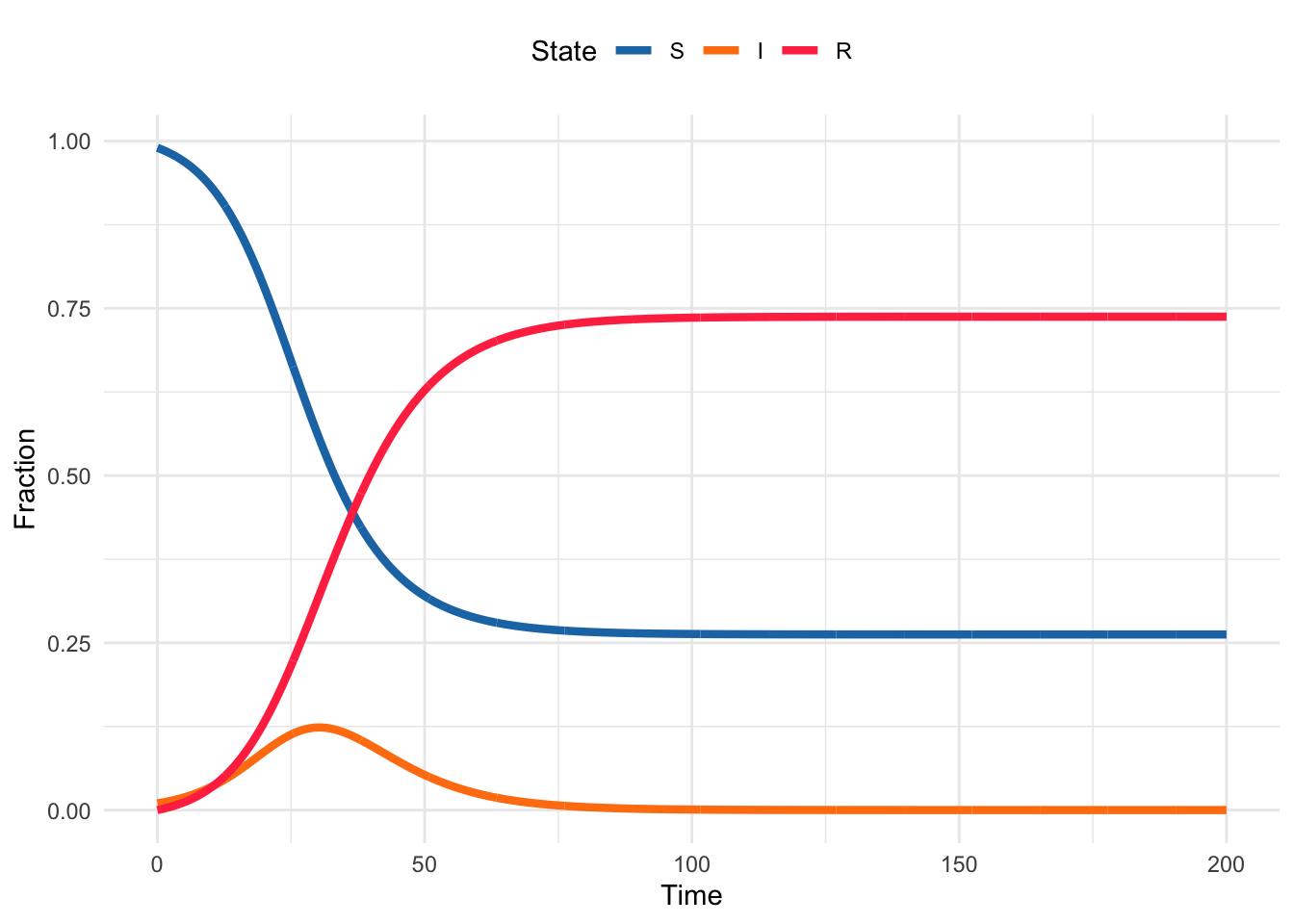

3.4.2 Commenting the code

For this part of the exercise, go through the basic SIR code and add comments to each section of code explaining what it does. To get you started, we’ve added some comments to the creating of the dataframe object sir_sol_df between lines 32-62 in the code block above, as some of the functions used there are a bit more complicated.

Note

Normally you would not use nearly as extensive comments. Here, we’ve gone overboard to help you understand what each line does, as some may not be familiar with all the functions used. We’ve also broken up the comments into multiple lines so that it is easier to read on this website. For your code that you view in RStudio (or some other text editor), use one line per sentence of the comment i.e., start a new comment line after each period.

Generally, you want to use comments to explain why you are doing something, not what you are doing. Sometimes that is unavoidable (e.g., you had to look up how to do a particular thing in R and need the hints to be able to understand the code), but try to stick to this guideline where possible.

As you’re going through the code, if you don’t understand what a particular function does, try looking up the documentation for it! You can do this by clicking on the function within the website (as described in the intro), or by typing ?function_name into the R console (Google also is your friend here!).

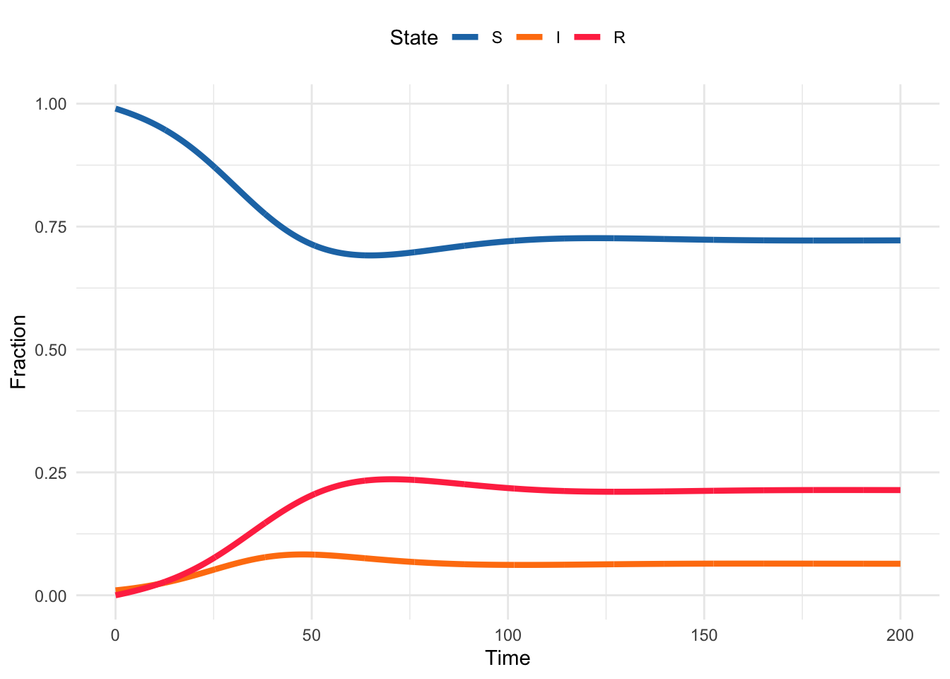
3.4.3 Adding in demographics

Now we have a better sense of how the code works, let’s add in some demographic structure. To recreate the demographic model from the interactive plot in Section 3.1, we just need to add births and deaths to the system.

Recall the equations for the demographic model:

\[ \begin{aligned} \frac{dS}{dt} &= \mu N - \beta S I - \mu S \\ \frac{dI}{dt} &= \beta S I - \gamma I - \mu I \\ \frac{dR}{dt} &= \gamma I - \mu R \end{aligned} \tag{3.1}\]

3.4.3.1 Create a new R script called 01_demographic-sir.R and copy the code from S01_basic-sir.R into it.

3.4.3.2 Rename the function sir_model() to demographic_sir_model() in your new script (S01_demographic-sir.R).

3.4.3.3 Adapt the function demographic_sir_model() to match the above equations (Equation 3.1).

SET

birth rate = 0.05

3.4.3.4 Rename the variables to reflect that we are now working with a demographic model, not the basic SIR model.

3.4.3.5 Plot the results of your demographic model. Does it look like this?

3.4.3.6 Update the comments in your code to reflect the changes you have made.

3.5 Exercise Solutions

Note

Here, we’re using the roxygen2 package to create the comments for the functions we’ve created, i.e., sir_model <- function(...). This provides a consistent framework for commenting functions, and if we wanted, we could use the comments to create documentation for our functions. The main benefit for our purposes is that the framework allows us to quickly understand exactly what the function does, as well as the context it should be used in.

3.5.1 Section 3.4.2: Commented basic SIR code

Code

# Load packages
library(tidyverse)
library(deSolve)

# Set the ggplot2 theme
theme_set(theme_minimal())

#' Basic SIR model
#'
#' A basic SIR model with no demographic structure to be used in deSolve
#'
#' @param time deSolve passes the time parameter to the function.
#' @param state A vector of states.
#' @param params A vector of parameter values .
#' @param ... Other arguments passed by deSolve.
#'
#' @return A deSolve matrix of states at each time step.
#' @examples
#' sir_params <- c(transmission = 0.3, duration = 6)
#' sir_init_states <- c(S = 0.99, I = 0.01, R = 0)
#' sim_times <- seq(0, 200, by = 0.1)
#' 
#' sir_sol <- deSolve::ode(
#'    y = sir_init_states,
#'    times = sim_times,
#'    func = sir_model,
#'    parms = sir_params
#' ))
sir_model <- function(time, state, params, ... ){
  # Extract parameters for cleaner calculations
  transmission <- params["transmission"]
  recovery <- 1 / params["duration"]

  # Extract states for cleaner calculations
  S <- state["S"]
  I <- state["I"]
  R <- state["R"]

  # Differential equations of the SIR model
  dSdt <- -transmission * S * I
  dIdt <- (transmission * S * I) - (recovery * I)
  dRdt <- recovery * I

  # Return a list whose first element is a vector of the
  # state derivatives - must be in the same order as the
  # state vector (S, I, R)
  return(list(c(dSdt, dIdt, dRdt)))
}

# Create the parameter, initial state, and time vectors
sir_params <- c(transmission = 0.3, duration = 6)
sir_init_states <- c(S = 0.99, I = 0.01, R = 0)
sim_times <- seq(0, 200, by = 0.1)

# Solve the SIR model with deSolve's ode() function
sir_sol <- deSolve::ode(
  y = sir_init_states,
  times = sim_times,
  func = sir_model,
  parms = sir_params
)

# Turn the output from the ODE solver into a tibble (dataframe)
# so we can manipulate and plot it easily
sir_sol_df <- as_tibble(sir_sol) %>%
  # Convert all columns to numeric (they are currently type
  # deSolve so will produce warnings when plotting etc)
  mutate(
    # Rather than repeatedly type the same function for every
    # column, use the across() function to apply the function
    # to a selection of columns
    across(
      # The cols argument takes a selection of columns to apply
      # a function to. Here, we want to apply the as.numeric()
      # function to all columns, so we use the function
      # everything() to select all columns.
      .cols = everything(),
      .fns = as.numeric
    )
  ) %>%
  # Convert the dataframe from wide to long format, so we have a
  # column for the time, a column for the state, and a column
  # for the proportion of the population in that state at that
  # time
  pivot_longer(
    # Don't pivot the time column
    cols = -time,
    names_to = "state",
    values_to = "proportion"
  ) %>%
  # Update the state column to be a factor, so the plot will
  # show the states in the correct order
  mutate(state = factor(state, levels = c("S", "I", "R")))

# Save the colors to a vector
SIRcolors <- c(S = "#1f77b4", I = "#ff7f0e", R = "#FF3851")

# Plot the results
ggplot(sir_sol_df, aes(x = time, y = proportion, color = state)) +
  geom_line(linewidth = 1.5) +
  scale_color_manual(values = SIRcolors) +
  labs(
    x = "Time",
    y = "Fraction",
    color = "State"
  ) +
  theme(legend.position = "top")

3.5.2 Section 3.4.3: Commented demographic SIR code

Code

# Load packages
library(tidyverse)
library(deSolve)

# Set the ggplot2 theme
theme_set(theme_minimal())

#' Demographic SIR model
#'
#' An SIR model with births and deaths (constant pop) to be used in deSolve
#'
#' @param time deSolve passes the time parameter to the function.
#' @param state A vector of states.
#' @param params A vector of parameter values .
#' @param ... Other arguments passed by deSolve.
#'
#' @return A deSolve matrix of states at each time step.
#' @examples
#' sir_params <- c(transmission = 0.3, duration = 6, birth_rate = 0.05)
#' sir_init_states <- c(S = 0.99, I = 0.01, R = 0)
#' sim_times <- seq(0, 200, by = 0.1)
#' 
#' sir_sol <- deSolve::ode(
#'    y = sir_init_states,
#'    times = sim_times,
#'    func = sir_demog_model,
#'    parms = sir_params
#' ))
sir_demog_model <- function(time, state, params, ... ){
  transmission <- params["transmission"]
  recovery <- 1 / params["duration"]
  birth_rate <- params["birth_rate"]

  S <- state["S"]
  I <- state["I"]
  R <- state["R"]

  dSdt <- birth_rate -transmission * S * I - (birth_rate * S)
  dIdt <- (transmission * S * I) - (recovery * I) - (birth_rate * I)
  dRdt <- (recovery * I) - (birth_rate * R)

  return(list(c(dSdt, dIdt, dRdt)))
}

# Create the parameter, initial state, and time vector
sir_demog_params <- c(transmission = 0.3, duration = 6, birth_rate = 0.05)
sir_init_states <- c(S = 0.99, I = 0.01, R = 0)
sim_times <- seq(0, 200, by = 0.1)

# Solve the SIR model with deSolve's ode() function
sir_demog_sol <- deSolve::ode(
  y = sir_init_states,
  times = sim_times,
  func = sir_demog_model,
  parms = sir_demog_params
)

# Turn the output from the ODE solver into a tibble (dataframe)
# so we can manipulate and plot it easily
sir_demog_sol_df <- as_tibble(sir_demog_sol) %>%
  # Convert all columns to numeric (they are currently type
  # deSolve so will produce warnings when plotting etc)
  mutate(
    # Rather than repeatedly type the same function for every
    # column, use the across() function to apply the function
    # to a selection of columns
    across(
      # The cols argument takes a selection of columns to apply
      # a function to. Here, we want to apply the as.numeric()
      # function to all columns, so we use the function
      # everything() to select all columns.
      .cols = everything(),
      .fns = as.numeric
    )
  ) %>%
  # Convert the dataframe from wide to long format, so we have a
  # column for the time, a column for the state, and a column
  # for the proportion of the population in that state at that
  # time
  pivot_longer(
    # Don't pivot the time column
    cols = -time,
    names_to = "state",
    values_to = "proportion"
  ) %>%
  # Update the state column to be a factor, so the plot will
  # show the states in the correct order
  mutate(state = factor(state, levels = c("S", "I", "R")))

# Save the colors to a vector
SIRcolors <- c(S = "#1f77b4", I = "#ff7f0e", R = "#FF3851")

# Plot the results
ggplot(sir_demog_sol_df, aes(x = time, y = proportion, color = state)) +
  geom_line(linewidth = 1.5) +
  scale_color_manual(values = SIRcolors) +
  labs(
    x = "Time",
    y = "Fraction",
    color = "State"
  ) +
  theme(legend.position = "top")